Age Wizard¶

Download all the Jupyter notebooks from: https://github.com/HeloiseS/hoki/tree/master/tutorials

Initial imports¶

[1]:

from hoki.age.wizard import AgeWizard
import hoki
import pandas as pd
import matplotlib.pyplot as plt
import numpy as np
from hoki.load import unpickle
import hoki.constants as hc

%matplotlib inline
plt.style.use('tuto.mplstyle')

A systematic ageing method¶

Motivation¶

One of the classic methods for ageing clusters is to fit isochrones to observational data in Colour-Magnitude Diagrams (CMDs) or in Hertzsprung-Russel Diagrams (HRDs).

There are a number of issues with this ubiquitous technique though:

Fitting is usually done by eye
They only take into account single stars
It cannot be used if your sample only contains a few sources

Our goal is to provide a method that answers all of the issues metioned above

How it works¶

By matching the observed properties of your sources to the BPASS models you can find the most likely age of a location on |the HRD/CMD.

Drawing

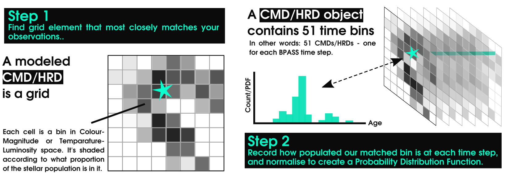
If all your sources belong to the same region, you can then combine the PDFs of your individual sources to find the age PDF of the whole cluster.

All of this can be done step by step using the chain find_coordinates() -> calculate_pdfs -> multiply_pdfs(), or you could simply use AgeWizard() which handles this pipeline and facilitates loading in the models.

Note: In this tutorial we will focus on AgeWizard().

Remember to exercise caution in your interpretation¶

This is true of all methods but it is worth repeating. This technique helps you get to the answer, but it doesn’t give you the answer.

The most likely age of the matching location is not necessarily the age of your source - as we’ll see below Helium Stars created through binary interactions and envelope stripping are found at similar locations as WR stars but at different ages.

Ages from Hertzsprung-Russell Diagram¶

First, we need some observational data to compare to our models.

AgeWizard() expects a pandas.DataFrame. If you want to use the HRD capabilities you will need to provide a logT and a logL column: * logT: log10 of the stellar effective temperature * logL: log10 of the stellar luminosity in units of Solar Luminosities

Additionally, your DataFrame will ideally contain a name column with the name of the sources you’re working on. If you don’t provide one, AgeWizard() will make it’s own sources names: source1, source2, etc…

Data source: McLeod et al. 2019, Stevance et al. in prep.

[2]:

stars = pd.DataFrame.from_dict({'name':np.array(['Star1','Star2','Star3','Star4',
                                                 'Star5','Star6','Star7','Star8','Star9',
                                                 'Star10','Star11','Star12','Star13','Star14',
                                                 'WR1', 'WR2']),
                                'logL':np.array([5.0, 5.1, 4.9, 5.9, 5.0, 5.4, 4.3, 5.7, 4.5, 4.5,
                                                 4.9, 4.5, 4.3, 4.5, 5.3, 5.3]),
                                'logT':np.array([4.48, 4.45, 4.46, 4.47, 4.48, 4.53, 4.52, 4.52, 4.52,
                                                 4.56, 4.46, 4.52, 4.52, 4.52, 4.9, 4.65])})

Now we initialise our AgeWizard(). Each instance corresponds to one model and one model only: i.e. 1 IMF and 1 metalicity.

If we want to have a look at 2 different metallicities for example, we can just instanciate AgeWizard twice:

[3]:

agewiz006 = AgeWizard(obs_df=stars, model='./data/hrs-bin-imf135_300.z006.dat')
agewiz008 = AgeWizard(obs_df=stars, model='./data/hrs-bin-imf135_300.z008.dat')

[---INFO---] AgeWizard Starting
[--RUNNING-] Initial Checks
Stack has been reset
[-COMPLETE-] Initial Checks
[---INFO---] ERROR_FLAG=None / No errors detected
[---INFO---] Distributions Calculated Successfully
[---INFO---] Distributions Normalised to PDFs Successfully
[---INFO---] AgeWizard Starting
[--RUNNING-] Initial Checks
Stack has been reset
[-COMPLETE-] Initial Checks
[---INFO---] ERROR_FLAG=None / No errors detected
[---INFO---] Distributions Calculated Successfully
[---INFO---] Distributions Normalised to PDFs Successfully

During instanciation, the observations and models are matched and the age PDFs are calculated. They are summarised in a pandas.DataFrame that you can access as follows.

[4]:

agewiz006.pdfs.head(15)

[4]:

name	Star1	Star2	Star3	Star4	Star5	Star6	Star7	Star8	Star9	Star10	Star11	Star12	Star13	Star14	WR1	WR2
0	0.000000	0.000000	0.000000	1.298460e-11	0.000000	0.000000	0.025706	5.594794e-11	0.021803	0.000000e+00	0.000000	0.021803	0.025706	0.021803	0.000000e+00	0.107142
1	0.000000	0.000000	0.000000	0.000000e+00	0.000000	0.000000	0.036928	0.000000e+00	0.030149	0.000000e+00	0.000000	0.030149	0.036928	0.030149	0.000000e+00	0.004603
2	0.000000	0.000000	0.000000	0.000000e+00	0.000000	0.000000	0.046310	0.000000e+00	0.035243	0.000000e+00	0.000000	0.035243	0.046310	0.035243	0.000000e+00	0.006676
3	0.000000	0.000000	0.000000	0.000000e+00	0.000000	0.000000	0.058174	0.000000e+00	0.052005	7.820472e-08	0.000000	0.052005	0.058174	0.052005	0.000000e+00	0.012032
4	0.000000	0.000000	0.000654	0.000000e+00	0.000000	0.000000	0.081692	0.000000e+00	0.057408	1.012331e-04	0.000654	0.057408	0.081692	0.057408	0.000000e+00	0.003365
5	0.000000	0.000000	0.015330	7.629112e-01	0.000000	0.000000	0.063921	4.216232e-03	0.074740	9.941176e-07	0.015330	0.074740	0.063921	0.074740	4.525980e-08	0.009378
6	0.075321	0.011572	0.142812	1.100859e-01	0.075321	0.003387	0.078904	2.914504e-01	0.086366	1.476180e-04	0.142812	0.086366	0.078904	0.086366	0.000000e+00	0.000145
7	0.238335	0.430026	0.233166	8.879082e-02	0.238335	0.558455	0.135883	4.335802e-01	0.093930	1.763084e-03	0.233166	0.093930	0.135883	0.093930	2.155362e-14	0.015148
8	0.295138	0.348300	0.279178	2.892240e-02	0.295138	0.345761	0.187286	1.529185e-01	0.147844	4.403392e-03	0.279178	0.147844	0.187286	0.147844	3.207127e-01	0.023512
9	0.324156	0.153717	0.267386	9.289685e-03	0.324156	0.044554	0.176904	8.005393e-02	0.204892	1.732683e-02	0.267386	0.204892	0.176904	0.204892	5.301331e-01	0.745544
10	0.023544	0.025031	0.023663	0.000000e+00	0.023544	0.032551	0.072708	3.722405e-02	0.165809	1.310383e-02	0.023663	0.165809	0.072708	0.165809	2.254815e-02	0.060667
11	0.016194	0.017432	0.015374	0.000000e+00	0.016194	0.011823	0.004711	5.566887e-04	0.006944	6.358691e-03	0.015374	0.006944	0.004711	0.006944	9.453766e-03	0.002344
12	0.017234	0.011523	0.014033	0.000000e+00	0.017234	0.003118	0.003887	0.000000e+00	0.006177	6.590932e-02	0.014033	0.006177	0.003887	0.006177	3.787228e-06	0.001189
13	0.008077	0.001189	0.006150	0.000000e+00	0.008077	0.000000	0.004152	0.000000e+00	0.006443	6.874719e-01	0.006150	0.006443	0.004152	0.006443	6.385924e-05	0.000039
14	0.000061	0.000322	0.001203	0.000000e+00	0.000061	0.000134	0.007283	0.000000e+00	0.003896	4.532046e-02	0.001203	0.003896	0.007283	0.003896	1.007283e-03	0.000000

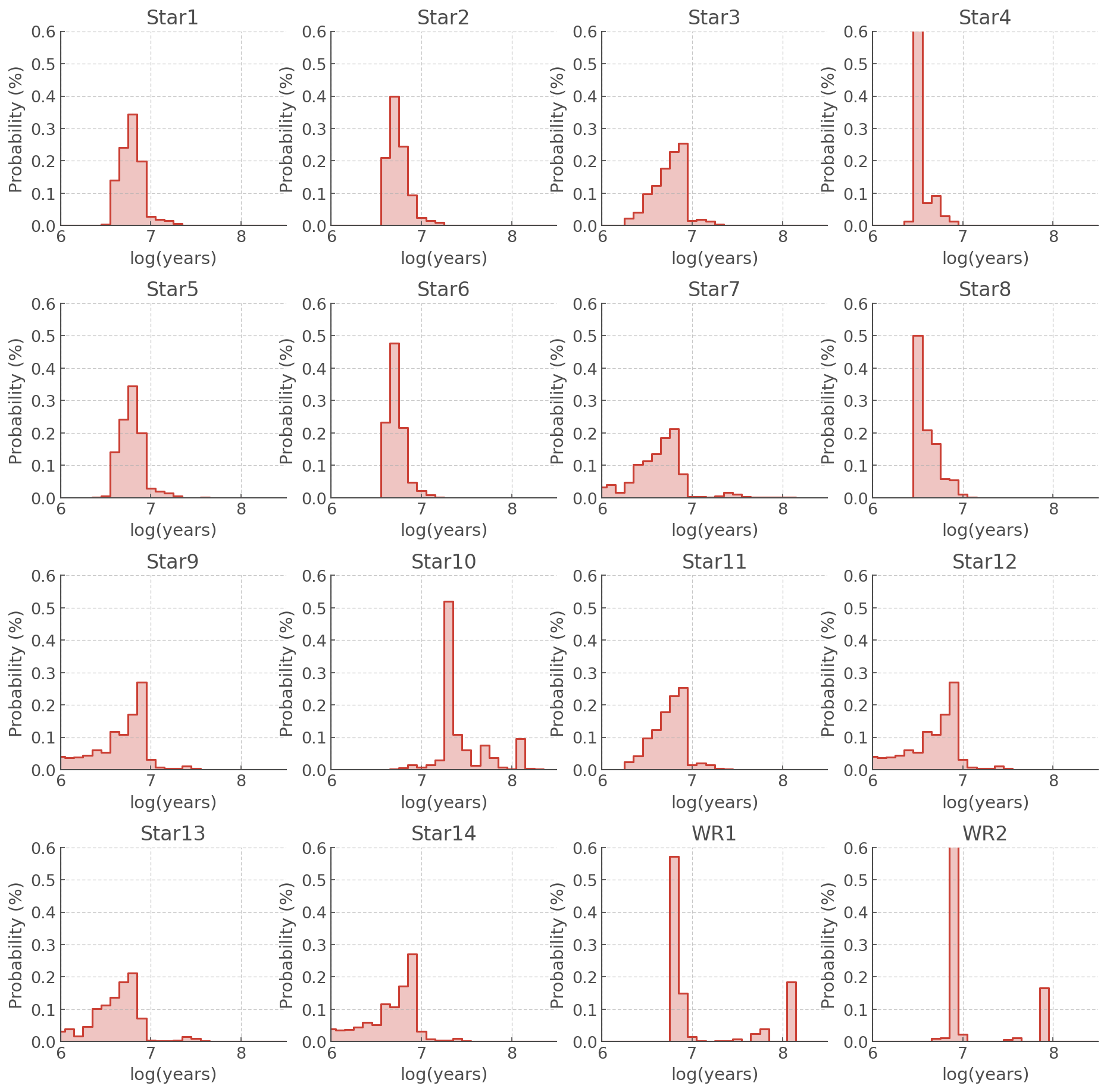
But those are just numbers… PDFs are meant to be plotted:

[5]:

def plot_all_pdfs(agewiz):
    # creating the figure
    f, ax = plt.subplots(4, 4, figsize=(15,15))
    plt.subplots_adjust(hspace=0.4)
    axes = ax.reshape(16)

    # We plot each star an individual axis
    for source, axis in zip(agewiz.sources, axes):

        # Plotting one PDF
        axis.step(hoki.BPASS_TIME_BINS, agewiz.pdfs[source],where='mid')
        axis.fill_between(hoki.BPASS_TIME_BINS, agewiz.pdfs[source], step='mid', alpha=0.3)

        # Labels and limits
        axis.set_title(source)
        axis.set_ylabel('Probability (%)')
        axis.set_xlabel('log(years)')
        axis.set_ylim([0,0.6])
        axis.set_xlim([6,8.5])

Age PDFs at z=0.006¶

[6]:

plot_all_pdfs(agewiz006)

Age PDFs at z=0.008¶

[7]:

plot_all_pdfs(agewiz008)

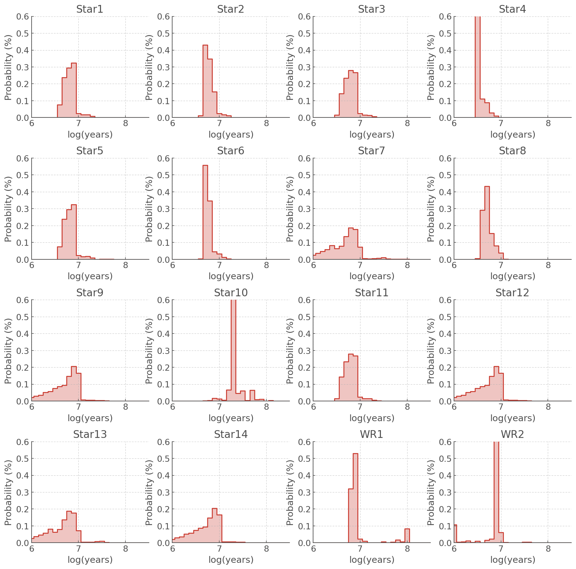
Most Likely Ages¶

The most likely age for each source is summarised by AgeWizard.most_likely_ages. This is returned as a numpy array.

[8]:

agewiz006.most_likely_ages

[8]:

array([6.9, 6.7, 6.8, 6.5, 6.9, 6.7, 6.8, 6.7, 6.9, 7.3, 6.8, 6.9, 6.8,
       6.9, 6.9, 6.9])

Different metallicities will give different results. In this example we summarise our results into a new DataFrame:

[9]:

most_likely_ages = pd.DataFrame.from_dict({'name': agewiz006.sources,
                                           'z006': agewiz006.most_likely_ages,
                                           'z008': agewiz008.most_likely_ages})

# Note that the attribute AgeWizard.sources is the list of names you provided, or if you didn't the ones it created

[10]:

most_likely_ages

[10]:

	name	z006	z008
0	Star1	6.9	6.8
1	Star2	6.7	6.7
2	Star3	6.8	6.9
3	Star4	6.5	6.5
4	Star5	6.9	6.8
5	Star6	6.7	6.7
6	Star7	6.8	6.8
7	Star8	6.7	6.5
8	Star9	6.9	6.9
9	Star10	7.3	7.3
10	Star11	6.8	6.9
11	Star12	6.9	6.9
12	Star13	6.8	6.8
13	Star14	6.9	6.9
14	WR1	6.9	6.8
15	WR2	6.9	6.9

IMPORTANT¶

The most_likely_ages (and most_likley_age, see below) tools do not give you a direct answer - they are a way to summarise the data and be used in your interpretation but please do not use these as a black box.

Looking at the PDFs plotted above and the table of most likely ages, we can see that a few stars stand out:

Star 4 has a lower (most likely) age than the rest of the sample
Star 10 has a higher (most likely) age than the rest of the sample
The WR PDFs show peaks beyond log(age/years) - which souldn’t be possible for WR stars.

All of these are discussed an interpreted in details in Stevance et al. (in prep). Star 4 is an example of a star that is probably the result of a merger and rejuvination, Star 10 is more likely to be on the young tail of the distribution and not as old as the most likley age implies, and the WR stars share their HRD locations with helium stars which appear at later times, which populate the later peak.

Plotting Aggregate Ages¶

If you are looking for the age of a whole population then you can ask AgeWizard to combine the PDFs it calcualted on initialisation. This is done with the method AgeWizard.calcualte_sample_pdfs().

It can be called as such and it will multiply all the PDFs, or you can provide a list of columns to ignore in the paramter not_you. You can also ask it to return the resulting PDF by setting return_df to True. If you don’t, it will store the result in AgeWizard.sample_pdf.

[11]:

# Returns None
agewiz006.calculate_sample_pdf()

[12]:

agewiz006.sample_pdf.head(10)

[12]:

	pdf
0	0.013998
1	0.010557
2	0.012814
3	0.017775
4	0.021274
5	0.072452
6	0.079372
7	0.189020
8	0.199454
9	0.233262

You can also quickly retrieve the most likely age of the whole sample from the PDF you just calculated using AgeWizard.most_likely_age.

[13]:

agewiz006.most_likely_age

[13]:

array([6.9])

[14]:

# Or return directly
agewiz008.calculate_sample_pdf(return_df=True).head(10)

[14]:

	pdf
0	0.011530
1	0.011737
2	0.009253
3	0.017201
4	0.030133
5	0.116927
6	0.117052
7	0.167216
8	0.201176
9	0.187655

[15]:

agewiz008.most_likely_age

[15]:

array([6.8])

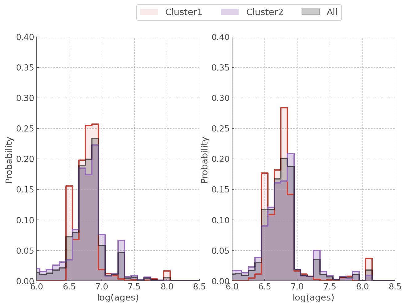
Down below we create a quick function to plot our aggregate ages for z=0.006 and z=0.008.

As an example of the

[16]:

cluster1_sources = ['Star1', 'Star2', 'Star3', 'Star4', 'WR1']
cluster2_sources = [item for item in agewiz006.sources if item not in cluster1_sources]

[17]:

def plot_aggregate_age(agewiz, ax):

    # Aggregate age PDF for all sources
    cluster12 = agewiz.calculate_sample_pdf(return_df=True).pdf

    # Aggregate age PDF for cluster1
    cluster1 = agewiz.calculate_sample_pdf(not_you=cluster2_sources, return_df=True).pdf

    # Aggregate age PDF for cluster2
    cluster2 = agewiz.calculate_sample_pdf(not_you=cluster1_sources, return_df=True).pdf



    ax.step(hoki.BPASS_TIME_BINS, cluster1, where='mid', alpha=1, lw=2)
    ax.fill_between(hoki.BPASS_TIME_BINS, cluster1, step='mid', alpha=0.1,  label='Cluster1')

    ax.step(hoki.BPASS_TIME_BINS, cluster2, where='mid', alpha=1, lw=2)
    ax.fill_between(hoki.BPASS_TIME_BINS,  cluster2, step='mid', alpha=0.3,  label='Cluster2')

    ax.step(hoki.BPASS_TIME_BINS, cluster12, where='mid',alpha=0.5, c='k', lw=2)
    ax.fill_between(hoki.BPASS_TIME_BINS,  cluster12, step='mid', alpha=0.2, label='All', color='k')


    ax.set_ylabel('Probability')
    ax.set_xlabel('log(ages)')

[18]:

f, ax = plt.subplots(ncols=2, nrows=1, figsize=(10,7))

plot_aggregate_age(agewiz006, ax[0])
plot_aggregate_age(agewiz008, ax[1])

for axis in ax:
    axis.set_ylim([0,0.4])
    axis.set_xlim([6,8.5])

# Cool legend
ax[0].legend(fontsize=14, loc='center right', bbox_to_anchor=(1.9, 1.1), ncol=3)

[18]:

<matplotlib.legend.Legend at 0x7f6ee56b3fd0>

Probability given an age range¶

The BPASS time bins are separated by 0.1 dex in log space (log(age/years) = 6.0, 6.1, 6.2, 6.3 etc..) and the PDFs for your individual sources will cover a range of BPASS time bins.

Consequently, giving a single age may not make a lot of sense. Also the PDFs will rarely, if ever, resemble a Gaussian distribution: that means that you can’t give an error bar in the “classical” sense.

Another interesting measure is the probability that the age of your star falls into a chosen age range. In this case our aggregate age is most likely to be between 6.7-6.9, so let’s investigate how likely it is for each individual star to fall in that range.

For that we use AgeWizard.calculate_p_given_age_range() which returns a Series containing the probabilities corresponding to each source.

[19]:

agewiz006.calculate_p_given_age_range([6.7, 6.9])

[19]:

name
Star1     0.857630
Star2     0.932043
Star3     0.779729
Star4     0.127003
Star5     0.857630
Star6     0.948770
Star7     0.500073
Star8     0.666553
Star9     0.446666
Star10    0.023493
Star11    0.779729
Star12    0.446666
Star13    0.500073
Star14    0.446666
WR1       0.850846
WR2       0.784204
dtype: float64

We can collate those in one single DataFrame

[20]:

p_ages_679 = pd.DataFrame.from_dict({'name': agewiz006.sources,
                                     'z006': agewiz006.calculate_p_given_age_range([6.7,6.9]),
                                     'z008': agewiz008.calculate_p_given_age_range([6.7,6.9])})

[21]:

p_ages_679

[21]:

	name	z006	z008
name
Star1	Star1	0.857630	0.784335
Star2	Star2	0.932043	0.737951
Star3	Star3	0.779729	0.659319
Star4	Star4	0.127003	0.134967
Star5	Star5	0.857630	0.784335
Star6	Star6	0.948770	0.738479
Star7	Star7	0.500073	0.469008
Star8	Star8	0.666553	0.278005
Star9	Star9	0.446666	0.549145
Star10	Star10	0.023493	0.023109
Star11	Star11	0.779729	0.659319
Star12	Star12	0.446666	0.549145
Star13	Star13	0.500073	0.469008
Star14	Star14	0.446666	0.549145
WR1	WR1	0.850846	0.721919
WR2	WR2	0.784204	0.789553

To learn more about how we use and interpret this statistic, you can checkout Stevance et al 2020

Errors on L and T¶

But what if my luminosity and temperature values have errors?

AgeWizard in the hoki.age.wizard subpackage (in hoki v1.6) can take care of that. The legacy version cannot.

To show you how it runs we’re going to use a made up example (these are the numbers I use in the unitest). The errors have to be given in the following columns ``logL_err`` and ``logT_err``.

GIVE THE 1 SIGMA ERRORS
If your errors are asymmetric – pick the largest value.

[22]:

stars_SYM = pd.DataFrame.from_dict({'name': np.array(['118-1', '118-2', '118-3', '118-4']),
                                    'logL': np.array([5.0, 5.1, 4.9, 5.9]),
                                    'logL_err': np.array([0.1, 0.2, 0.1, 0.1]),
                                    'logT': np.array([4.48, 4.45, 4.46, 4.47]),
                                    'logT_err': np.array([0.1, 0.2, 0.1, 0.1]),
                                    })

How are the errors taken into account?¶

Basically bootstrapping. Each data point is thought of as a gaussian distribution centered on the value with standard deviation the error your gave (that is why I ask you to give AgeWizard the 1 sigma level).

Then for each data point is drawn from that distribution and the individual age PDFs are calculated as usual. This process is repeated n_samples times and the individual pdfs are then combined.

Finally you can get the age PDF of the whole cluster (or sample) by doinmg the usual AgeWizard.calculate_sample_pdf().

[23]:

errwiz = AgeWizard(stars_SYM, model='./data/hrs-bin-imf135_300.z006.dat', nsamples=200)
errwiz.calculate_sample_pdf()

[---INFO---] AgeWizard Starting
[--RUNNING-] Initial Checks
Stack has been reset
[-COMPLETE-] Initial Checks
[---INFO---] ERROR_FLAG=SYM / Strictily symmetric errors detected
None
[---INFO---] Distributions Calculated Successfully
[---INFO---] Distributions Normalised to PDFs Successfully

[24]:

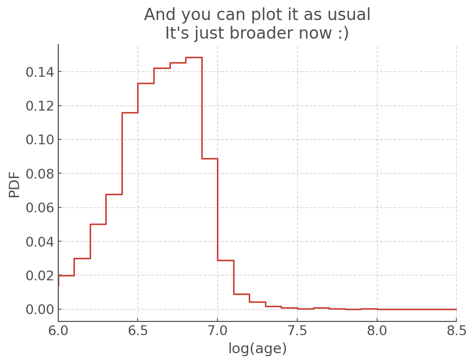
plt.step(errwiz.t, errwiz.sample_pdf.pdf)
plt.xlabel('log(age)')
plt.ylabel('PDF')
plt.xlim([6,8.5])
plt.title("And you can plot it as usual\nIt's just broader now :)")

[24]:

Text(0.5, 1.0, "And you can plot it as usual\nIt's just broader now :)")

Ages from Colour-Magnitude Diagram¶

In this section we will see how we can use AgeWizard on a Colour-Magnitude Diagram (CMD). It is essentially the same as for the HR Diagrams but you will be giving AgeWizard a hoki.CMD object instead of a hoki.HRDiagram object.

This example is taken from Brennan et al. 2021b where we look at the neighbourhood of AT2016jbu to try and infer the age.

Loading data¶

To help you we’ve attached a couple of pre-made CMDs. You can make your own following the CMD.ipynb tutorial, or if you don’t want to download 50GB of stellar models you can send me an email and for the low price of adding me to your author list I will make them for you.

In addition to the models we need to download the data and turn observed magnitudes into absolute magnitudes by removing the distance modulus and the extinction.

[25]:

# The BPASS synthetic CMDs
f435cmd = unpickle(path='./data/F435_F555.pckl')
f555cmd = unpickle(path='./data/F555_F814.pckl')


# The observed data
cmd_obs = pd.read_csv('./data/phot_150pc.dat')
cmd_obs.replace([99.999, 9.999], np.nan, inplace=True) # cleaning up bad values

# Absolute magnitudes
# - 31.6 is the distance modulus to NGC242 and the other value is extinction see Brennan et al. 2021
F435 = cmd_obs.F435W - 31.6 - 0.732
F555 = cmd_obs.F555W - 31.6 - 0.579
F814 = cmd_obs.F814W - 31.6 - 0.309

# we add teh absolute magnitudes to the dataframe, it'll be useful later
cmd_obs['abs_F435'] = F435
cmd_obs['abs_F555'] = F555
cmd_obs['abs_F814'] = F814

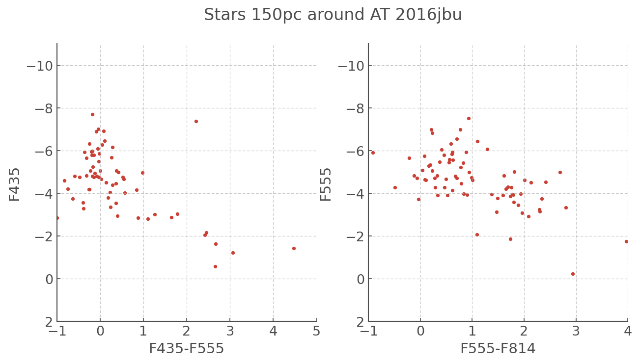
[26]:

fig, ax = plt.subplots(ncols = 2, figsize=(10,5))

ax[0].scatter(F435-F555, F435)
ax[0].set_xlim([-1,5.0])
ax[0].set_ylim([2,-11])
ax[0].set_xlabel('F435-F555')
ax[0].set_ylabel('F435')

ax[1].scatter(F555-F814, F555)
ax[1].set_xlim([-1,4])
ax[1].set_ylim([2,-11])
ax[1].set_xlabel('F555-F814')
ax[1].set_ylabel('F555')

plt.suptitle('Stars 150pc around AT 2016jbu', fontsize=16)

[26]:

Text(0.5, 0.98, 'Stars 150pc around AT 2016jbu')

Putting constraints on the age of a population using AgeWizard¶

The CMDs are very scattered and it might seem like there isn’t much we can do, but trust the process… Let’s take a look at them with some BPASS CMDs plotted underneath

[27]:

f, ax = plt.subplots(ncols=2,figsize=(12,5))

myplot = f435cmd.plot(log_age=7.5, loc=ax[0]) # Here you can chose the time bin you want to plot.
myplot.scatter(F435-F555, F435)
myplot.set_xlim([-1,5.0])
myplot.set_ylim([2,-11])

myplot = f555cmd.plot(log_age=7.5, loc=ax[1]) # Here you can chose the time bin you want to plot.
myplot.scatter(F555-F814, F555)
myplot.set_xlim([-1,4])
myplot.set_ylim([2,-11])

/home/fste075/hoki/hoki/cmd.py:348: MatplotlibDeprecationWarning: You are modifying the state of a globally registered colormap. In future versions, you will not be able to modify a registered colormap in-place. To remove this warning, you can make a copy of the colormap first. cmap = copy.copy(mpl.cm.get_cmap("Greys"))
  colMap.set_under(color='white')

[27]:

(2.0, -11.0)

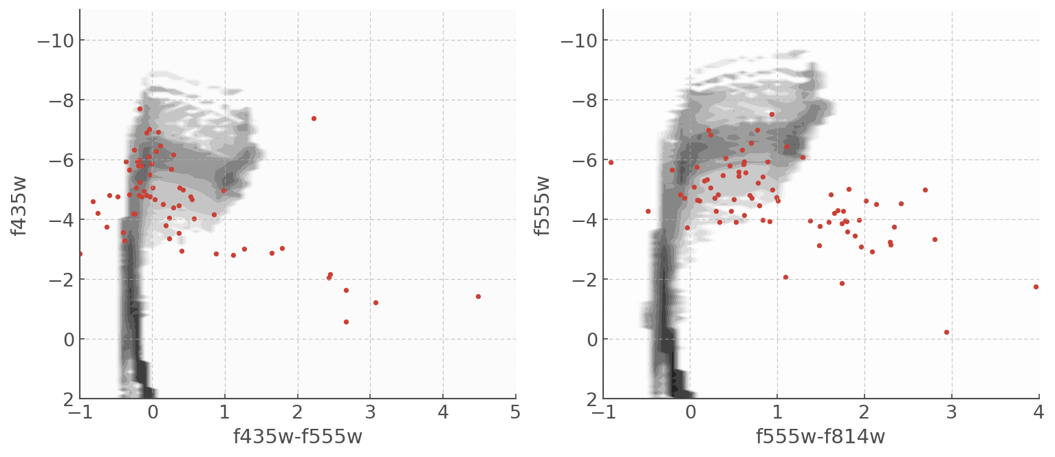
The scatter will make it hard (impossible) to get a neat and precise age estimate, but we can put constraints on the age and exclude age ranges that really don’t fit the data. Creating the age pdf is very useful for that.

The first thing we will do is cut-off some of the more dificult data - we see that below an absolute mag of -4 the data slides unexpectedly to the right. That horizontal displacement is not from stellar evolution so we’re going to apply a luminosity cut-off and only pick the stars brighter than -4.

Luminosity cut-off¶

[28]:

## we crop our dataframe based on the absolute magnitude and the cut-off we chose
cmd_obs_crop=cmd_obs[(cmd_obs.abs_F435<-4) & (cmd_obs.abs_F555<-4)]

# we can also create columns for the colours.
cmd_obs_crop['F555-F814'] = cmd_obs_crop.abs_F555-cmd_obs_crop.abs_F814
cmd_obs_crop['F435-F555'] = cmd_obs_crop.abs_F435-cmd_obs_crop.abs_F555

<ipython-input-28-93413fe7f498>:5: SettingWithCopyWarning:
A value is trying to be set on a copy of a slice from a DataFrame.
Try using .loc[row_indexer,col_indexer] = value instead

See the caveats in the documentation: https://pandas.pydata.org/pandas-docs/stable/user_guide/indexing.html#returning-a-view-versus-a-copy
  cmd_obs_crop['F555-F814'] = cmd_obs_crop.abs_F555-cmd_obs_crop.abs_F814
<ipython-input-28-93413fe7f498>:6: SettingWithCopyWarning:
A value is trying to be set on a copy of a slice from a DataFrame.
Try using .loc[row_indexer,col_indexer] = value instead

See the caveats in the documentation: https://pandas.pydata.org/pandas-docs/stable/user_guide/indexing.html#returning-a-view-versus-a-copy
  cmd_obs_crop['F435-F555'] = cmd_obs_crop.abs_F435-cmd_obs_crop.abs_F555

AgeWizard¶

Now we can give all that to AgeWizard! We need to create two instances one for each CMD. We can then combine their results later.

NOTE: ``AgeWizard`` expects the observational data to have at least two columns with names ``mag`` and ``col``.

[29]:

##### CMD1 - F555 F814
# we drop the NaN values we used to mark the bad measurements
obs_df1=cmd_obs_crop[['abs_F555','F555-F814' ]].dropna()

# AgeWizard needs specific column names
obs_df1.columns=['mag','col']
agewiz1 = AgeWizard(obs_df1, model=f555cmd)

# Calculate the Age PDF of the whole sample from the individual age pdfs
agewiz1.calculate_sample_pdf()

[---INFO---] AgeWizard Starting
[--RUNNING-] Initial Checks
[-COMPLETE-] Initial Checks
[---INFO---] ERROR_FLAG=None / No errors detected
[---INFO---] Distributions Calculated Successfully
[---INFO---] Distributions Normalised to PDFs Successfully

/home/fste075/hoki/hoki/age/wizard.py:47: HokiFormatWarning: We expect the name of sources to be given in the 'name' column. If I can't find names I'll make my own ;)
  warnings.warn("We expect the name of sources to be given in the 'name' column. "
/home/fste075/hoki/hoki/age/utils.py:421: HokiUserWarning: No source names given so I'll make my own
  warnings.warn("No source names given so I'll make my own", HokiUserWarning)

[30]:

##### CMD2 - F435 F555
obs_df2=cmd_obs_crop[['abs_F435','F435-F555' ]].dropna()
obs_df2.columns=['mag','col']
agewiz2 = AgeWizard(obs_df2, model=f435cmd)

# Calculate the Age PDF of the whole sample from the individual age pdfs
agewiz2.calculate_sample_pdf()

[---INFO---] AgeWizard Starting
[--RUNNING-] Initial Checks
[-COMPLETE-] Initial Checks
[---INFO---] ERROR_FLAG=None / No errors detected
[---INFO---] Distributions Calculated Successfully
[---INFO---] Distributions Normalised to PDFs Successfully

/home/fste075/hoki/hoki/age/wizard.py:47: HokiFormatWarning: We expect the name of sources to be given in the 'name' column. If I can't find names I'll make my own ;)
  warnings.warn("We expect the name of sources to be given in the 'name' column. "
/home/fste075/hoki/hoki/age/utils.py:421: HokiUserWarning: No source names given so I'll make my own
  warnings.warn("No source names given so I'll make my own", HokiUserWarning)

[31]:

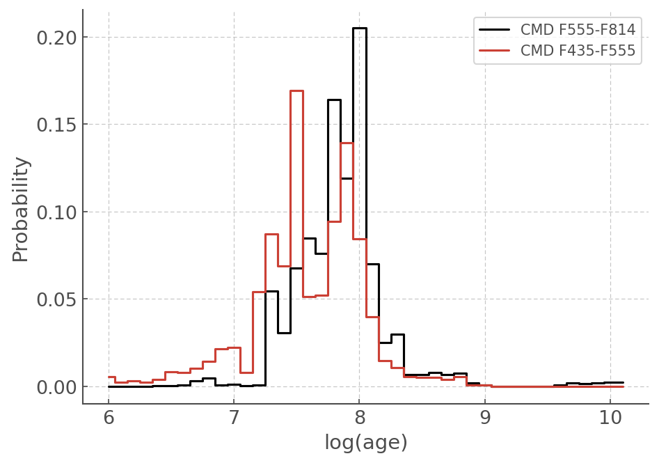
plt.step(agewiz1.t[:42], agewiz1.sample_pdf[:42], where='mid', c='k', label='CMD F555-F814')
plt.step(agewiz2.t[:42], agewiz2.sample_pdf[:42], where='mid',  label='CMD F435-F555')
plt.legend()

plt.ylabel('Probability')
plt.xlabel('log(age)')

[31]:

Text(0.5, 0, 'log(age)')

Combine the PDFs from the two CMDs¶

[32]:

# creates a new data frame with the final, combined, age pdf
combined_pdf = 0.5*(agewiz1.sample_pdf+agewiz2.sample_pdf)
# adds the time axis (x axis) to the index instead of having a range from 0 to 51 - eases plotting.
combined_pdf.index = agewiz2.t

[33]:

plt.step(combined_pdf.index , combined_pdf, where='mid', lw=2,color='crimson')
plt.fill_between(combined_pdf.index.values, combined_pdf.pdf, step='mid', color='crimson',lw=3,
                 alpha=0.2, zorder=0.2)
plt.xlim([6,9.3])
plt.ylim([0.000001,0.16])
plt.ylabel('Probability')
plt.xlabel('log(age)')
#plt.savefig('pdf_AgeWizard')

[33]:

Text(0.5, 0, 'log(age)')

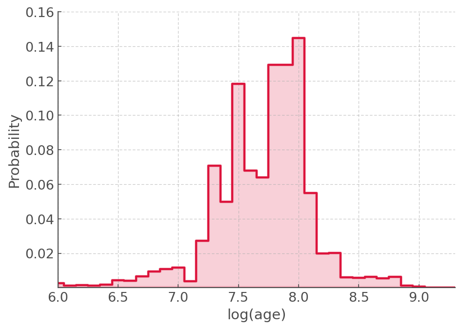
Age constraint¶

The PDF is very broad because the data is very scattered but the young ages are in a very low probably region.

We can quantify this by adding up the first 10 bins (10 Million years) and see how much probability is in it:

[34]:

proba_less_than_10Myr = combined_pdf.iloc[:10].sum().values[0]*100

[35]:

f"The probability that this population is less than 10 Myrs if {round(proba_less_than_10Myr,2)} percent"

[35]:

'The probability that this population is less than 10 Myrs if 4.37 percent'