Complex Model Search

Download all the Jupyter notebooks from: https://github.com/HeloiseS/hoki_tutorials

Initial Imports

import pandas as pd
import matplotlib.pyplot as plt
from hoki import load
from time import time
import gc

plt.style.use('./tuto.mplstyle')

Introduction

The BPASS outputs contain a lot of information that is pretty much ready for analysis and can be quickly loaded through hoki (e.g. HR Diagrams, star counts etc…)

But if you’re looking to match your observation to specific stellar models present in BPASS, say a binary system with primary ZAMS 9 \(M_{\odot}\) and absolute F814w magnitude = X, then you will need to explore the large library of BPASS stellar models to get those evolution tracks.

The best way to go about that is to compile all the relevant data (i.e. the IMFs and metallicities you want, for single or binary models) into one or multiple DataFrames that can then be saved into binary files. Loading data from binary files is much faster and it means you won’t have to compile your data frome text files multiple times. In this tutorial we will use pre-compiled DataFrames - if you want to learn how to make your own (but you probably won’t need to), check the ModelDataCompiler tutorial.

Downloading pre-compiled DataFrames

I have already compiled all of the BPASS stellar models for the fiducial IMF (Kroupa 1.35 maximum mass = 300 solar masses) into 26 DataFrames (one for each fo the 13 metallicities times 2 for the binay and single star models).

You can find the full data set here (just download what you need).

Model Search

Here we’ll demonstrate how to find BPASS models that match a simple set of observational data. We are using two HST magnitudes: F435W=-7.33, F814W=-8.46.

We’ll crop the data step by step and give a few tips and tricks along the way.

Loading the Data

For this particular exercise we are interested in a “SN” progenitor in a binary system - we assume solar metallicity, but if you have Z information, use whatever is closest.

Note: The required pickle file is NOT included in the tutorial repository because it’s too large. You’ll have to download it yourself.

all_models_z020=pd.read_pickle('./models_z020_bin_v221.pkl')

Let’s take a look at what we have:

all_models_z020

	?	AM_bin	B	B2	C	CO_core1	DAM	DM1A	DM1R	DM1W	...	z	z2	filenames	model_imf	types	mixed_imf	mixed_age	initial_BH	initial_P	z
0	-0.30896	4.83652e+49	-6.217291	99.0	0.003460	0.0	3.16506e+43	0.0	0.0	8.89633e-14	...	-5.494487	99.0	NEWSINMODS/z020/sneplot-z020-65	0.0778658	-1	0	0	NaN	NaN	020
1	-0.30896	4.83641e+49	-6.185996	99.0	0.003460	0.0	1.92552e+42	0.0	0.0	9.15485e-14	...	-5.457620	99.0	NEWSINMODS/z020/sneplot-z020-65	0.0778658	-1	0	0	NaN	NaN	020
2	-0.30897	4.83641e+49	-6.169761	99.0	0.003460	0.0	1.60184e+42	0.0	0.0	9.24452e-14	...	-5.440918	99.0	NEWSINMODS/z020/sneplot-z020-65	0.0778658	-1	0	0	NaN	NaN	020
3	-0.30897	4.83641e+49	-6.153298	99.0	0.003460	0.0	1.39289e+42	0.0	0.0	9.31861e-14	...	-5.423736	99.0	NEWSINMODS/z020/sneplot-z020-65	0.0778658	-1	0	0	NaN	NaN	020
4	-0.30897	4.83641e+49	-6.136751	99.0	0.003460	0.0	1.23073e+42	0.0	0.0	9.38489e-14	...	-5.406273	99.0	NEWSINMODS/z020/sneplot-z020-65	0.0778658	-1	0	0	NaN	NaN	020
...	...	...	...	...	...	...	...	...	...	...	...	...	...	...	...	...	...	...	...	...	...
2674010	-0.36221	2.27212e+48	19.097040	99.0	0.003439	0.0	0.1228691-243	0.0	0.0	0.3168876-307	...	15.096950	99.0	NEWSINMODS/z020/sneplot-z020-0.6	43.7266	3	0	0	NaN	NaN	020
2674011	-0.36221	2.27212e+48	19.189880	99.0	0.003439	0.0	0.1255959-243	0.0	0.0	0.3168876-307	...	15.140240	99.0	NEWSINMODS/z020/sneplot-z020-0.6	43.7266	3	0	0	NaN	NaN	020
2674012	-0.36221	2.27212e+48	19.289070	99.0	0.003439	0.0	0.1282466-243	0.0	0.0	0.3168876-307	...	15.183800	99.0	NEWSINMODS/z020/sneplot-z020-0.6	43.7266	3	0	0	NaN	NaN	020
2674013	-0.36221	2.27212e+48	19.395370	99.0	0.003439	0.0	0.1305542-243	0.0	0.0	0.3168876-307	...	15.227470	99.0	NEWSINMODS/z020/sneplot-z020-0.6	43.7266	3	0	0	NaN	NaN	020
2674014	-0.36221	2.27212e+48	19.509870	99.0	0.003439	0.0	0.1317481-243	0.0	0.0	0.3168876-307	...	15.271070	99.0	NEWSINMODS/z020/sneplot-z020-0.6	43.7266	3	0	0	NaN	NaN	020

2674015 rows × 102 columns

That’s 2,503,198 rows and 100 columns.

Note that there aren’t 2.5 million models: Each model has between 100 and 400 rows (roughly) that contain the time evolution of each column. It’s still a lot of models though, but about 2 orders of magnitude fewer than the number of rows.

Chopping off the bulk of models we don’t need

Before we match our magnitudes, there are a lot of models that are irrelevant to what we are doing that we can get rid of right off the bat.

Binaries only

Something important to note is that the BPASS binary models contain single stars. Binaries are important, but they are introduced in a proportion similar to what has been observationally determined (see the BPASS manual for more information or just go to Moe and Die Stefano 2017).

Since we only care about the binary star models, we can remove most of the 5 types - chekc the manual for full descriptions but here is a wuick reminder: - -1: Signle - 0: Merger before MS - 1: Normal Primary - 2: Normal Secondary - 3: Single Secondary - 4: QHE (Quasi Homogeneous Evolution) Secondary (only for low mtallicities)

all_models_z020.types.unique()

array([-1, 0, 1, 2, 3], dtype=object)

We only want binary so let’s create a smaller DataFrame with only these models (types 1 and 2):

only_binaries=all_models_z020[(all_models_z020.types==2) | (all_models_z020.types==1)].reset_index()

only_binaries

	index	?	AM_bin	B	B2	C	CO_core1	DAM	DM1A	DM1R	...	z	z2	filenames	model_imf	types	mixed_imf	mixed_age	initial_BH	initial_P	z
0	216919	-0.00411	1.28449e+49	-9.090588	120.7212	0.003460	0.00000	5.21861e+43	0.0	-0.000000e+00	...	-8.441809	118.5559	NEWBINMODS/NEWBINMODS/z020/sneplot-z020-300-0.4-1	0.0694137	1	0	0	NaN	NaN	020
1	216920	-0.00412	1.28437e+49	-9.027635	120.7212	0.003460	0.00000	1.4804e+43	0.0	-0.000000e+00	...	-8.369311	118.5559	NEWBINMODS/NEWBINMODS/z020/sneplot-z020-300-0.4-1	0.0694137	1	0	0	NaN	NaN	020
2	216921	-0.00412	1.28425e+49	-8.939427	120.7212	0.003460	0.00000	1.18282e+43	0.0	-0.000000e+00	...	-8.277122	118.5559	NEWBINMODS/NEWBINMODS/z020/sneplot-z020-300-0.4-1	0.0694137	1	0	0	NaN	NaN	020
3	216922	-0.00412	1.28401e+49	-8.835626	120.7212	0.003460	0.00000	7.6132e+43	0.0	-0.000000e+00	...	-8.171609	118.5559	NEWBINMODS/NEWBINMODS/z020/sneplot-z020-300-0.4-1	0.0694137	1	0	0	NaN	NaN	020
4	216923	-0.00443	1.2669e+49	-8.894129	120.7212	0.003460	0.00000	2.47932e+45	0.0	-0.000000e+00	...	-8.231492	118.5559	NEWBINMODS/NEWBINMODS/z020/sneplot-z020-300-0.4-1	0.0694137	1	0	0	NaN	NaN	020
...	...	...	...	...	...	...	...	...	...	...	...	...	...	...	...	...	...	...	...	...	...
2120614	2624805	-0.03574	1.19768e+47	-2.930821	99.0000	0.000403	1.09695	4.41908e+41	0.0	-2.643257e-14	...	-6.752302	99.0000	NEWBINMODS/NEWSECMODS/z020_2/sneplot_2-z020-7-...	0.0364456	2	0	0	NaN	NaN	020
2120615	2624806	-0.03574	1.1972e+47	-3.199305	99.0000	0.000340	1.10326	5.06699e+41	0.0	-2.588900e-14	...	-6.852680	99.0000	NEWBINMODS/NEWSECMODS/z020_2/sneplot_2-z020-7-...	0.0364456	2	0	0	NaN	NaN	020
2120616	2624807	-0.03574	1.19664e+47	-3.330151	99.0000	0.000453	1.11016	2.23323e+41	0.0	-5.042884e-14	...	-6.990517	99.0000	NEWBINMODS/NEWSECMODS/z020_2/sneplot_2-z020-7-...	0.0364456	2	0	0	NaN	NaN	020
2120617	2624808	-0.03574	1.19661e+47	-3.332807	99.0000	0.000463	1.11028	2.9105e+38	0.0	-5.188726e-14	...	-6.995630	99.0000	NEWBINMODS/NEWSECMODS/z020_2/sneplot_2-z020-7-...	0.0364456	2	0	0	NaN	NaN	020
2120618	2624809	-0.03574	1.19661e+47	-3.332807	99.0000	0.000463	1.11028	2.9105e+38	0.0	-5.188726e-14	...	-6.995630	99.0000	NEWBINMODS/NEWSECMODS/z020_2/sneplot_2-z020-7-...	0.0364456	2	0	0	NaN	NaN	020

2120619 rows × 103 columns

One thing we need to be very careful about is memory. We don’t want to fill up our RAM. If you do that in a jupyter notebook, the kernel will crash, saving you from having to reboot.

If you fill up your RAM in a script without fail-safes, your computer will freeze and you will most likely have to reboot.

So when creating new DataFrames like we just did, it’s very important to kill the previous, uncropped DataFrame to free that memory.

Before we kill it, let’s see how much memory the binary models for z020 were taking up:

f"This one DataFrame is taking up {round(sum(all_models_z020.memory_usage())/1e9, 2)} GB of RAM"

'This one DataFrame is taking up 2.18 GB of RAM'

Let’s free that up:

del all_models_z020
gc.collect()
# We need this because python loves to hold onto old memories it doesn't need anymore.
# gc.collect() forces it to release memory allocations is doesn't need anymore.
# not sure it works great in Jupyter notebooks, but if you run this in a script it should help.

281

Select your columns

Okay so now that we’ve selected the types of interest, we can select the information that we actually care about.

The available columns are:

print(list(only_binaries.columns))

['index', '?', 'AM_bin', 'B', 'B2', 'C', 'CO_core1', 'DAM', 'DM1A', 'DM1R', 'DM1W', 'DM2A', 'DM2R', 'DM2W', 'FUV', 'H', 'H2', 'Halpha', 'He_core1', 'I', 'I2', 'J', 'J2', 'K', 'K2', 'M1', 'M2', 'MC1', 'MFe1', 'MH1', 'MHe1', 'MMg1', 'MN1', 'MNe1', 'MO1', 'MSi1', 'MTOT', 'Mej_SN', 'Mej_superSN', 'Mej_weakSN', 'Mrem_SN', 'Mrem_superSN', 'Mrem_weakSN', 'N', 'NUV', 'Ne', 'O', 'ONe_core1', 'P_bin', 'R', 'R2', 'U', 'U2', 'V', 'V-I', 'V2', 'X', 'Y', 'age', 'envelope_binding_E', 'f300w', 'f300w2', 'f336w', 'f336w2', 'f435w', 'f435w2', 'f450w', 'f450w2', 'f555w', 'f555w2', 'f606w', 'f606w2', 'f814w', 'f814w2', 'g', 'g2', 'i', 'i2', 'log(L1)', 'log(L2)', 'log(R1)', 'log(R2)', 'log(T1)', 'log(T2)', 'log(a)', 'mixedimf', 'modelimf', 'r', 'r2', 'star_binding_E', 'timestep', 'u', 'u2', 'z', 'z2', 'filenames', 'model_imf', 'types', 'mixed_imf', 'mixed_age', 'initial_BH', 'initial_P', 'z']

For this particular case, we’re going to select the following columns. Note that filenames is essential because it is basically the ID for each model (since there is pretty much 1 text file per modelled system).

cols =['age','M1','log(L1)', 'log(T1)', 'log(R1)',
       'M2','log(L2)', 'log(T2)', 'log(R2)',
       'P_bin','log(a)', 'f435w','f555w', 'f814w', 'filenames']

# Now we replace our DataFrame by one that contains only the columns we care about
only_binaries=only_binaries[cols].reset_index()

only_binaries.head()

	index	age	M1	log(L1)	log(T1)	log(R1)	M2	log(L2)	log(T2)	log(R2)	P_bin	log(a)	f435w	f555w	f814w	filenames
0	0	0.000	300.0000	6.81875	4.58633	1.76008	119.9997	6.23655	4.67478	1.29114	0.0274287	2.165326	-9.142474	-8.853167	-8.555243	NEWBINMODS/NEWBINMODS/z020/sneplot-z020-300-0.4-1
1	1	1239.810	299.9159	6.82043	4.59835	1.73689	119.9926	6.23662	4.67476	1.29121	0.0274428	2.165444	-9.079781	-8.787302	-8.484336	NEWBINMODS/NEWBINMODS/z020/sneplot-z020-300-0.4-1
2	2	2014.764	299.8613	6.82159	4.61140	1.71137	119.9850	6.23667	4.67476	1.29125	0.027451	2.165509	-8.991781	-8.697519	-8.393105	NEWBINMODS/NEWBINMODS/z020/sneplot-z020-300-0.4-1
3	3	3403.802	299.7607	6.82033	4.62595	1.68164	119.9709	6.23676	4.67475	1.29131	0.0274659	2.165627	-8.888180	-8.592647	-8.288321	NEWBINMODS/NEWBINMODS/z020/sneplot-z020-300-0.4-1
4	4	105333.700	292.4715	6.81136	4.61411	1.70085	118.9247	6.24327	4.67409	1.29588	0.0285882	2.174324	-8.946525	-8.652020	-8.347613	NEWBINMODS/NEWBINMODS/z020/sneplot-z020-300-0.4-1

Okay so now we are working with a DataFrame of much more reasonable size 386,150 rows instead of 2.5 million.

Now let’s match our magnitudes.

Matching Magnitudes and Period

Now we want to find which models can reproduce our observed magnitudes and potential period We use a conservative error=0.5, you can use your own.

#targets
F435W=-7.33
F435W_err=0.5 #arbitrary
F814W=-8.46
F814W_err=0.5 #arbitrary
P=45
P_err=15

Before we apply conditions, we need to be careful, to the types of the columns we’re going to rely on for the conditions. I know from trying this that the periods are not all floats - some numbers get messed up (not enough bits because the exponent is too big??) and look like this: -0.8122210+122 - which should be -0.8122210e+122.

Anyways, these numbers are going to be plus infinities we don’t want anyway.

Thankfully ``pandas`` has all the resources we need to elegantly take care of that!

# This turns our P_bin column into floats, and if a cell cannot be turned into a float, a NaN is put in its place
only_binaries['P_bin']=pd.to_numeric(only_binaries['P_bin'],errors='coerce')

# Condition 1: Selects rows where the f435 column is within 0.5 mag or our target
condition1 = (only_binaries.f435w<F435W+F435W_err) & (only_binaries.f435w>F435W-F435W_err)

# Condition 2: Selects rows where the f814 column is within 0.5 mag or our target
condition2 = (only_binaries.f814w<F814W+F814W_err) & (only_binaries.f814w>F814W-F814W_err)

# Condition3: Select the period
condition3 = (only_binaries.P_bin*365.25<P+P_err) & (only_binaries.P_bin*365.25>P-P_err)

# We need ALL conditions to be met for a row to be selected
mag_match=only_binaries[condition1 & condition2 & condition3]

Something to keep in mind is that a star can stay within our magnitude targets for a while and so give multiple hits (rows). What we want is a list of unique models that satisfy our query at some point in their lifetime.

Thankfully, it’s very easy in pandas:

matching_model_list=mag_match.filenames.unique().tolist()

f"There are {len(matching_model_list)} matching models"

'There are 264 matching models'

Now that we have a list of models that match, we need to retrieve their whole stellar evolution journey, not just the one that matches our magnitudes (otherwise our HR Diagram would look kinda weird).

Let’s make a new DataFrame:

# If this syntax seems odd, you might want to check out the following links:
# https://python-3-patterns-idioms-test.readthedocs.io/en/latest/Comprehensions.html
# https://chrisalbon.com/python/data_wrangling/pandas_selecting_rows_on_conditions/

model_match_df=only_binaries[[True if model in matching_model_list
                                 else False
                                 for model in only_binaries.filenames]]

# And we get rid of stuff we don't need
del only_binaries
gc.collect()

769

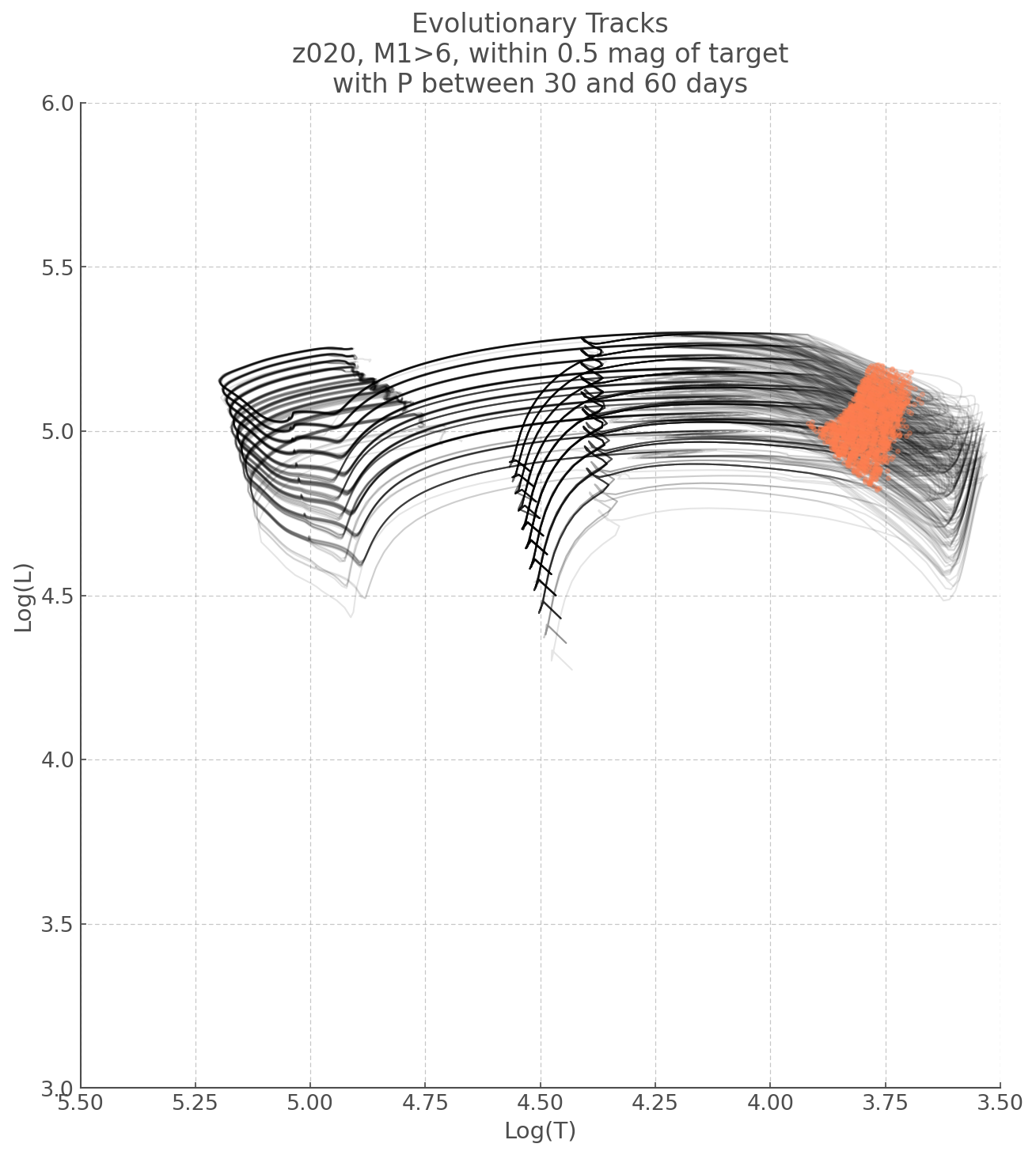
Plotting Evolutionary Tracks

Now that we have the models we care about, let’s have a look at where they lie on an HR Diagram and what kind of lifestyle they have.

As any task implemented in python there are many ways you could do this, here is mine: * 1) First we iterate over each model ID (filename) and record the evolution of its Temperature, Luminosity, and Magnitudes in respective lists. * 2) We’ll then collate these lists into a list of lists for each property (i.e. one list for temperature evolutions, one list for luminosity evolutions, etc..) * 3) We can then iterate over the length of our Lists of lists and plot them accordingly.

Note you could combine step 3 with step 2 but I’d rather have the main lists saved so I can re-use them if I want.

# Initiate Main Lists
logT_list=[]
logL_list=[]
f435w_list=[]
f814w_list=[]

# Iterate over each model
for model in matching_model_list:

    # Data Frame containing solely the evolution of this one model
    model_df = model_match_df[model_match_df.filenames==model]

    # Putting the T, L and mag ecolution in temp lists
    logT, logL, f435w, f814w = model_df['log(T1)'].values, model_df['log(L1)'].values, model_df.f435w.values, model_df.f814w.values

    # Appending these temp lists to our Master Lists.
    logT_list.append(logT)
    logL_list.append(logL)
    f435w_list.append(f435w)
    f814w_list.append(f814w)

### And now we plot!

plt.figure(figsize=(10,11))

# Iterating over the length of our Master Lists (they all have the same length)
for i in range(len(logT_list)):
    # This is just easier later when we apply a mask
    logT_i, logL_i = logT_list[i], logL_list[i]

    # Plot L Vs T
    plt.plot(logT_i, logL_i, alpha=0.1, c='k', lw=1)

    # We are also plotting where in the stellar evolution, our tracks produce the desired magnitudes
    # These are the same conditions we had earlier
    condition1 = (f435w_list[i]<F435W+F435W_err) & (f435w_list[i]>F435W-F435W_err)
    condition2 = (f814w_list[i]<F814W+F814W_err) & (f814w_list[i]>F814W-F814W_err)
    # Our mask is a combination of those two conditions
    mask=condition1 & condition2
    # We use a scatter plot to show the masked L and T combinations
    plt.scatter(logT_i[mask], logL_i[mask], zorder=1000, c='coral', alpha=0.3)

# Just some limits - also flips the Temperature axis, to make this an HRD
plt.xlim([5.5, 3.5])
plt.ylim([3,6])

#Labels
plt.ylabel('Log(L)')
plt.xlabel('Log(T)')

plt.title('Evolutionary Tracks\nz020, M1>6, within 0.5 mag of target\nwith P between 30 and 60 days')

Text(0.5, 1.0, 'Evolutionary Tracks\nz020, M1>6, within 0.5 mag of target\nwith P between 30 and 60 days')

---

YOU’RE ALL SET!

I hope you found this tutorial useful. If you encountered any problems, or would like to make a suggestion, feel free to open an issue on hoki GitHub page here or on the hoki_tutorials GitHub there.