Complex Stellar Histories
Download all the Jupyter notebooks from: https://github.com/HeloiseS/hoki_tutorials
Initial Imports
[1]:
import matplotlib.pyplot as plt
import numpy as np
from hoki.constants import *

%matplotlib inline
plt.style.use('tuto.mplstyle')
In this tutorial you will learn:
The Stellar Formation History class,
SFH, and its attributesUsing
CSPEventRateto generate event rates for complex stellar populations
BPASS contains simple stellar populations (all co-eval) with a total of \(10^{6}\) M\(_\odot\) at for a given metallicity and imf. While this is a valid assumption for some populations, others can have a more complex stellar formation history and metallicity evolution. Therefore, we introduce the hoki.csp package. This package allows for the creation of more complex stellar populations using the BPASS populations.
Stellar Formation History
Many of the standard stellar formation histories (SFH) are included in hoki.csp.sfh package. These SFH are generated using the SFH class, which always takes a time array and a string as inputs. The time array determines the sampling of the time domain, while the string determines the type of SFH to use. Each available formation history has a unique string identifier. A list of all available formation histories and their identifiers can be found in the hoki documentation. #[link]!!
[https://heloises.github.io/hoki/manual.html#module-hoki.csp.sfh]
If you wish to us a built-in SFH, you will also needs to parse a dictionary containing the necessary parameters and their values. A comprehensive list of these can also be found in the documentation.
In this example we load in three of the built-in SFH:
Burst
Constant
Log Normal
SFH class
[2]:
from hoki.csp.sfh import SFH
[3]:
# Creating 100 time points from age 0 to the current age of the Universe
time_axis = np.linspace(0,HOKI_NOW, 100)

# Instanciating a Burst SFH
burst = SFH(time_axis, "b", {"T0": 1e9, "constant":10})

# Instanciating a constant SFH
constant = SFH(time_axis, "c", {"constant":1})

# Instanciating a log_normal SFH
log_normal = SFH(time_axis, 'ln', {"constant":10, "tau":0.8, "T0":1})
/Users/mbri637/Documents/code/hoki/hoki/csp/sfh.py:166: RuntimeWarning: divide by zero encountered in log
  - ((np.log(self.time_axis/1e9) - self.params['T0']) ** 2) / (2 * self.params['tau'] ** 2)))
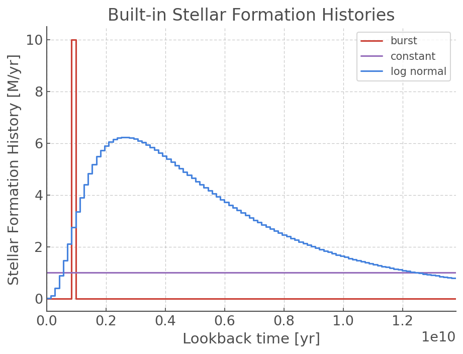
Now that we have create SFH instances, we can take a look at their shapes by plotting them. Like other hoki objects (HRDiagram, CMD), the SFH class comes with its own plotting method: SFH.plot().
[4]:
burst.plot(label="burst")
constant.plot(label="constant")
log_normal.plot(label="log normal")
plt.title("Built-in Stellar Formation Histories")
plt.ylabel("Stellar Formation History [M/yr]")
plt.xlabel("Lookback time [yr]")
plt.xlim(0, 13.8e9)
plt.legend()
plt.show()
/Users/mbri637/Documents/code/hoki/hoki/csp/sfh.py:170: MatplotlibDeprecationWarning: Adding an axes using the same arguments as a previous axes currently reuses the earlier instance.  In a future version, a new instance will always be created and returned.  Meanwhile, this warning can be suppressed, and the future behavior ensured, by passing a unique label to each axes instance.
  sfh_plot = plt.subplot(loc)
Custom SFH
Besides the built-in stellar formation histories, it’s possible to make your own stellar formation history.
The identifier "custom" allows for the input of a value array, sfh_arr, which contains the star formation rates associated with each time bin parsed in time_axis(that means it should be the same length). In this case, the parameter dictionary is not called and you don’t need to provide it.
[5]:
# Custom star formation history values
values = np.linspace(0,10,len(time_axis))

# Instanciation of our custom SFH object
custom = SFH(time_axis, "custom", sfh_arr=values)
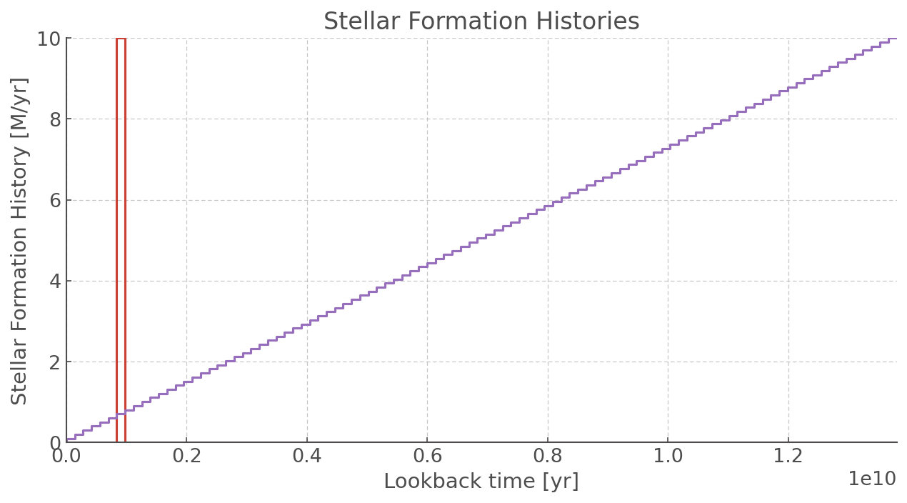
Let’s plot it to see what it looks like :)
[6]:
plt.figure(figsize=(10,5))
burst.plot()
custom.plot()
plt.title("Stellar Formation Histories")
plt.ylabel("Stellar Formation History [M/yr]")
plt.xlabel("Lookback time [yr]")
plt.xlim(0, 13.8e9)
plt.ylim(0,10)
plt.show()
/Users/mbri637/Documents/code/hoki/hoki/csp/sfh.py:170: MatplotlibDeprecationWarning: Adding an axes using the same arguments as a previous axes currently reuses the earlier instance.  In a future version, a new instance will always be created and returned.  Meanwhile, this warning can be suppressed, and the future behavior ensured, by passing a unique label to each axes instance.
  sfh_plot = plt.subplot(loc)
Event Rate calculations
By combining the BPASS populations with the complex SFH, it is possible to generate transient rates for the new populations. hoki provides the subpackage hoki.csp.eventrate for this purpose.
Initialisation of CSPEventRate
When initialising the CSPEventRate class, it loads and normalises the BPASS supernova files for all metallicities. Stored in a pandas.DataFrame, they are accessible using CSPEventRate.bpass_rates. The following event types are available from BPASS: [Ia, IIP, II, Ib, Ic, LGRB, PISNe, low_mass]
BPASS contains a selection of initial mass functions. To support all of them, the CSPEventRate class requires an imf identifier. These can be found in the class’s documentation.
! ! ! ! WARNING ! ! ! !
If you want to run the following cells you will to change the path_to_files to your local folder containing the BPASS supernova files. If you downloaded them straight off the google drive, it’ll probably have a name like bpass_v2.2.1_imf135_300
[7]:
from hoki.csp.eventrate import CSPEventRate
[8]:
path_to_files = "../BPASS_hoki_dev/bpass_v2.2.1_imf135_300"
imf_identifier = "imf135_300"
ER_CSP = CSPEventRate(path_to_files, imf_identifier, binary=True)
Calculating event rates
After initialising the class, the event rates for complex stellar populations can be calculated using the following functions: - CSPEventRate.at_time - CSPEventRate.over_time
Both take the same 3 parameters: - Description of the SFH - Descriptoin of the Metallicity Evolution - An array containing the event types to be calculated
Defining an SFH and metallicity evolution
We define a constant metallicity and stellar formation rate. The methods in CSPEventRate require the SFH and metallicity evolution to be provided as python callables (i.e something that can be called, i.e something that require brackets to work: myfunction()). It is also possible to use a SFH object as an input for the SFH evolution – it was designed to work with these :)
Here, we define two python functions describing the SFH and metallicity evolution. These have to be set to 0 if the age is older than the universe. We define the SFR to be constant at 1 and the metallicity to be constant at solar.
[9]:
def SFR_evolution(t):
    if t < HOKI_NOW:
        return 1.0
    else:
        return 0

def Z_evolution(t):
    return 0.0020
CSPEventRate.at_time
Input
In addition to the 3 standard input parameters, you need to provide the time at which you want the event rates calculated.
You can provide more than one SFH and metallicity histories, as described below
As an optional input, the sampling rate of the SFH and metallicity evolution can be given. The default sampling is set to 1000. This makes the calculation accurate and fast. If a negative number is given, the BPASS bins are used.
Output
The output an array, where each element corresponds to an SHF/metallicity history pair.
Each complex stellar population contains an array with the type of transient event as an identifier.
output[nr csp][event type]
[10]:
# calculate rate at LB = 0 Gyr
er_zero = ER_CSP.at_time(SFR_evolution, Z_evolution, ["Ia"], 0)
print("Event Rate now:", er_zero[0]["Ia"])

# calculate rate at LB = 10 Gyr
er_ten = ER_CSP.at_time(SFR_evolution, Z_evolution, ["Ia"], 10e9)
print("Event rate at 10 Gyr lookback time:", er_ten[0]["Ia"])

# High sampling event rate
er_high_sampling = ER_CSP.at_time(SFR_evolution, Z_evolution, ["Ia"], 10e9, 2000)

print("Event rate 1000 samples:", er_high_sampling[0]["Ia"])
Event Rate now: 0.0015103559493986228
Event rate at 10 Gyr lookback time: 0.0013245082839476612
Event rate 1000 samples: 0.0013273604259601117
It is also possible to input several SFH and metallicity evolutions in a single function call by inputting two lists of equal length. Each SFH will be associated with a metallicity evolution at the same index.
[11]:
er = ER_CSP.at_time([SFR_evolution, SFR_evolution],
                    [Z_evolution, Z_evolution],
                    ["Ia", "II"],
                    0)
print("First history, Ia rates:", er[0]["Ia"])
print("Second history, II rates:", er[1]["II"])
First history, Ia rates: 0.0015103559493986228
Second history, II rates: 0.0035807774002009902
Of course, it is also possible to provide a SFH object from hoki as an input.
[12]:
er = ER_CSP.at_time(constant,
                    Z_evolution,
                    ["Ia", "II"],
                    0)
print("Ia rates:", er[0]["Ia"])
print("II rates:", er[0]["II"])
Ia rates: 0.0015103573172394677
II rates: 0.0035807774002009902
CSPEventRate.over_time
This method splits the lookback time up into a chosen number of bins and calculates the event rate over the whole lookback time at once. Because the event rates over the full history of the universe is calculated, this method is more computationally intensive than CSPEventRate.at_time.
In addition to the 3 standard input parameters, this method requires you to provide a number of bins that determines the number of bins the complete lookback time is split into.
It has an optional argument, return_time_edges, that will return the time edges of the binning (in addition to the standard outputs).
[13]:
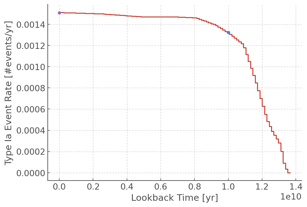
er_all, edges = ER_CSP.over_time([SFR_evolution], [Z_evolution], ["Ia"], 100, return_time_edges=True)
[14]:
plt.step(edges[:-1], er_all[0]["Ia"], where="pre")
plt.xlabel("Lookback Time [yr]")
plt.ylabel("Type Ia Event Rate [#events/yr]")
plt.plot(0, er_zero[0]["Ia"], "o")
plt.plot(10e9, er_ten[0]["Ia"], "o")
plt.show()
Grid Calculations: EventRates
Sometimes using a Python callable isn’t the right way to describe the stellar formation history, such as when working with simulations with stored data points. Therefore, it is also possible to provide a 2D grid (nr_sfhx13xN) as an SFH input. This matrix splits up each SFH into BPASS metallicity bins (13) per time point (N). The nr_sfh is always necesarry even when a single SFH grid is given.
The associated functions are:
CSPEventRate.grid_at_timeCSPEventRate.grid_over_time
Instead of taking a SFH and metallicity evolution both are separated to allow for material being created with different metallicities at the same time. Instead they need a time_points parameter describing what the lookback times of the 2D SFH are.
Note
Depending on your operating system, a “NumbaWarning about TBB threading” might appear when using the grid functions. This can be safely ignored.
EventRates
[15]:
# setup example 2D grid
time_points = np.linspace(0,HOKI_NOW, 101)
SFH_2D = np.zeros((13,len(time_points)), dtype=np.float64)
bpass_Z_index = np.array([np.argmin(np.abs(Z_evolution(i) - BPASS_NUM_METALLICITIES)) for i in time_points])
SFH_2D[bpass_Z_index] += np.array([SFR_evolution(i) for i in time_points])
Because our SFH_2D is only a 13x101 matrix we transform it into a 1x13x101 matrix for it to be used as input of our *.grid_at_time and *.grid_over_time functions.
[16]:
# Transform into (1x13xtime_points)
SFH_2D = SFH_2D.reshape((1,13,len(time_points)))
[17]:
# Event rate at lookback time t = 0
er_at_time_per_metallicity1 = ER_CSP.grid_at_time(SFH_2D, time_points, ["Ia"], 0)

# Event rate at lookback time t = 10 Gyr
er_at_time_per_metallicity2 = ER_CSP.grid_at_time(SFH_2D, time_points, ["Ia"], 10e9)

# The event rate over lookback time
er_over_time_per_metallicity, time_edges = ER_CSP.grid_over_time(SFH_2D, time_points, ["Ia"], 100, return_time_edges=True)
|----------------------------------------------------------------------------------------------------| 0.00%
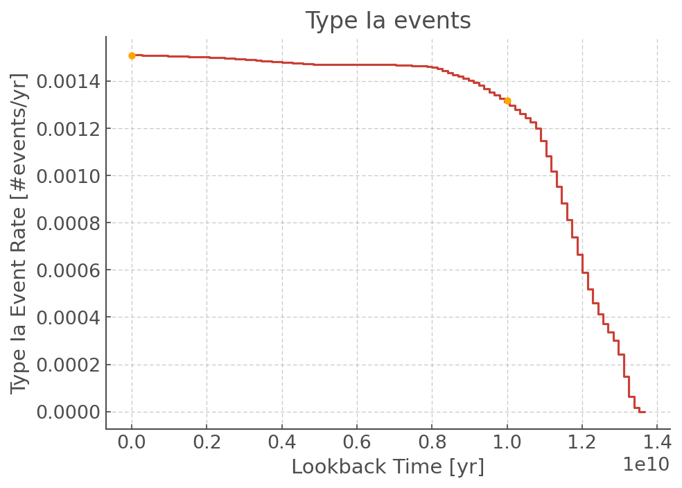
[18]:
# Sum select the first SFH and sum over the metallicity bins
er_over_time = er_over_time_per_metallicity[0].sum(axis=0)
er_at_time1 = er_at_time_per_metallicity1[0].sum(axis=0)
er_at_time2 = er_at_time_per_metallicity2[0].sum(axis=0)

plt.step(time_edges[:-1], er_over_time[0], label="Ia")
plt.plot(0, er_at_time1[0], "o", label="Ia", color="orange")
plt.plot(10e9, er_at_time2[0], "o", label="Ia", color="orange")
plt.title("Type Ia events")
plt.xlabel("Lookback Time [yr]")
plt.ylabel("Type Ia Event Rate [#events/yr]")
plt.show()